Exploratory analysis of datasets obtained from GEO

Damiano October 22, 2015 2 Comments

Gene Expression Omnibus (GEO) is an online public repository of functional genomics data. Information about GEO may be found at the following URL: http://www.ncbi.nlm.nih.gov/geo/info/faq.html. Briefly, GEO includes different types of datasets:

• GEO Profiles are curated datasets obtained from GEO DataSets. Not all original datasets are available as curated DataSets yet.
• GEODataSet (GDSxxx) contain information and genomics data corresponding to a specific biological sample. GDSxxx may be part of series representing a collection of biologically- and statistically-comparable samples processed using the same Platform
• GEO Series (GSExxx) are original submitter-supplied records summarizing a whole study

In order to explore and download GEO data from whitin R, we can use the following libraries:

library(GEOmetadb)
library(GEOquery)

Searching for a GEO Series of interest is very straightforward. It is possible perform an online search at the website http://www.ncbi.nlm.nih.gov/gds/. Alternatively, GEOmetadb.sqlite database may be saved locally and queried using the GEOmetadb package. Here, I am using GEOmetadb to retrieve the GEO identifier of a GEO Series of interest.

# Save a local copy of the GEOmetadb file
if(!file.exists(‘GEOmetadb.sqlite’)) getSQLiteFile()

 

# create a connection with the database

con <- dbConnect(SQLite(),’GEOmetadb.sqlite’)

 

# query GEO.db. In this case, my query is about uterine leiomyomas
gseList <- dbGetQuery(con,paste(“select gse, title from gse where”, “title like ‘%leiomyoma%'”,sep=” “))
gseList$title #vector containing the titles of the studies retrieved by our query
myGSE <- gseList[18,1] #GSE45188

Now that i have a GEO Series Id, I am using GEOquery to download the corresponding files.

gse <- getGEO(myGSE)

#gse is a list; you may want to check all items contained in it. In this case, there is just one ExpressionSet item that I retrieve in the following way:
eset <- gse[[names(gse)]]

Information about the genes (or the microarray probes) should be accessible via fData(eset). Gene expression data are accessible via exprs(eset). Phenotipic information, including the group (cancer vs. normal, for example) each sample belongs to, are accessible via pData(eset). Phenotipic Data contain very important information about samples and the experiment:

• microarray chip used
• sample preparation protocol / experimental procedures
• sample scaling, normalization and log conversion

It is important to check these information to make sure to correctly prepare data before proceeding with further analyses. If analyzing raw data, please check this post and prep your data first. ExpressionSet from GSE45188 is scaled, normalized and ready to undergo exploratory analysis.

head(pData(eset)) #sample groups as defined under the column characteristics_ch1.2
fac <- as.vector(pData(eset)$characteristics_ch1.2)
fac[grep(“myometr”,fac)]<-“myometrium”

fac[grep(“myometr”,fac, invert=TRUE)]<-“leiomyoma”

fac <- factor(fac, levels = c(“myometrium”,”leiomyoma”))

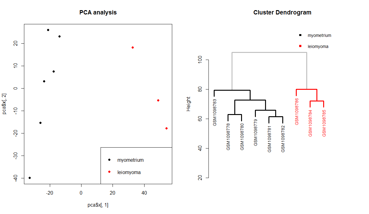
PCA analysis

A principal component analysis is a great way to start exploring the dataset. PCA analysis should confirm the presence of as many sample groups as defined in pData(eset). PCA analysis will help understand whether the dataset is usable or not. Other information in pData(eset) may also be used (instead of fac) for checking for major batch effects of confounding issues. PCA analysis in performed via the prcomp function. The values of the i-th principal component of each sample are accessible via pca$x[,i].

#pca analysis: are data clustered according to the sample groups?
pca <- prcomp(t(exprs(eset)))
plot(pca$x[,1],pca$x[,2],col=fac, main=”PCA analysis”, pch=16)
legend(“bottomright”,levels(fac),col=factor(levels(fac), levels = levels(fac)), pch=16)

Hierarchical clustering

Hierarchical clustering is a complementary approach to check whether the samples of a dataset may be clustered consistently with the groups as defined in pData(eset)$characteristics_ch1.2 (or in fac). Hierarchical clustering may be easily performed using the hclust function. Nice colored dendrograms based on hclust-class objects may be generated using the colorhcplot package.

library(colorhcplot)

hc <- hclust(dist(t(exprs(eset))))
colorhcplot(hc, fac, ax.low=20, ax.top = 120, tick.at = 20)

In this case, the results of the exploratory analysis are consistent with a very good dataset. Sample groups match perfectly with the clusters identified by the hierarcical clustering test and may be easily distinguished based on the first component of the PCA analysis. Sometimes, the results of the exploratory analysis are not very good. In those cases, it could be a good idea to try to identify sources of confounding and remove batch effects (if possible). If this doesn’t help, then it is better to search for another dataset.