RPKM calculation and relative gene expression quantification

Damiano May 4, 2015 0 Comments

RNAseq data may provide an estimate of the relative expression level of different genes in a sample or in a cell type. It is sufficient to compare RPKM (reads per kilobase trascript per million reads) values of the genes of interest. RPKM values may be calculated using the raw counts table.

RPKM i = (10 ^ 9) * (reads mapping on gene i) / ( ( total reads num ) * ( sum of exon lengths of gene i ) )

The list of genes to analyze is stored in the vector my_genes, while the raw counts table is loaded from a .csv file in the read_counts variable.

> head(read_counts)
            X   CTRL_1   CTRL_2   CTRL_3  siRNA_1  siRNA_2  siRNA_3
1 1/2-SBSRNA4       16       21       26       26       15       19
2        A1BG        3        2        4        4        5        2
3    A1BG-AS1        1        0        0        0        2        1
4        A1CF       14       21       19        5        4        5
5       A2LD1      147      129      139      184      189      201
6         A2M        0        1        3        0        1        2

As in this case I was interested in the relative expression levels of my genes of interest independently of the CTRL/siRNA treatment, the raw counts from the 6 different samples will be pooled together.

1. Retrieve the total exon length for each gene of interest

Total exon length is stored in a m-column matrix, where m is the number of gene of interest.

> #load required libraries
> library(org.Hs.eg.db)
> library(TxDb.Hsapiens.UCSC.hg19.knownGene)
> 
> my_genes<- c("GAPDH","XRCC6","CUL4B", "LEF1", "TCF7L2")
> read_counts <- read.csv("counts.csv", header = T, as.is=T)
> 
> #retrieve the total exon lenght of each gene of interest (feed symbol)
> gene_lookup <- select(org.Hs.eg.db,keys=my_genes, keytype="SYMBOL",columns=c("ENTREZID","SYMBOL","GENENAME","CHR","CHRLOC"))
> tx_lookup <- select(TxDb.Hsapiens.UCSC.hg19.knownGene, key=gene_lookup$ENTREZID, keytype="GENEID", columns= c("TXID","TXSTART","TXEND","EXONSTART","EXONEND","EXONID","TXSTRAND","EXONCHROM"))
> gene_IDs <- unique(tx_lookup$GENEID)
> results <- matrix(,ncol=length(my_genes), nrow=0)
> colnames(results) <- my_genes
> 
> results <- rbind(results,
+                  sapply (gene_IDs, (function(id){
+                    ex_ids <- unique(tx_lookup[which(tx_lookup$GENEID == id),"EXONID"])
+                    
+                    sum( 
+                      sapply(ex_ids, (function(ex){
+                        exons <- tx_lookup[which(tx_lookup$EXONID==ex &
+                                                   tx_lookup$GENEID==id),]
+                        as.numeric(as.matrix(exons)[1,"EXONEND"])-as.numeric(as.matrix(exons)[1,"EXONSTART"])
+                      })))
+                  }))
+ )
> rownames(results)[1] <- "all_exon_len"

2. Attach average raw count (calculated across all samples) to the results table

Average (across all 6 samples) counts were calculated for each gene of interest. Transcripts having no counts in one more CTRL sample & one or more siRNA sample, were imposed = 0.

> #define treatment groups (CTRL vs. siRNA)
> ctrls <- grep("CTRL",colnames(read_counts), ignore.case = T)
> treat <- grep("CTRL",colnames(read_counts), ignore.case = T, invert = T)
> treat <- treat[-which(colnames(read_counts)=="X")]
> 
> #Retrieve raw counts
> sel_counts <- read_counts[which(read_counts$X %in% my_genes),]
> results <- rbind(results,as.vector(
+   sapply(1:ncol(results),(function(r){
+     if (sum(sel_counts[which(sel_counts$X==colnames(results)[r]),ctrls]==0)>0 | sum(sel_counts[which(sel_counts$X==colnames(results)[r]),treat]==0)>0) {
+       0
+     } else {
+       mean(as.numeric(as.character(sel_counts[which(sel_counts$X==colnames(results)[r]),c(ctrls, treat)])))
+     }
+   }))
+ ))
> rownames(results)[2] <- "counts"

3. Calculate total number of reads

> #Attach total counts (across all samples)
> rw_reads<-which(
+   sapply(1:nrow(read_counts),(function(rrw){
+     if(sum(read_counts[rrw,ctrls]>0) == length(ctrls) |
+        sum(read_counts[rrw,treat]>0) == length(treat)) { T } else { F }
+   }))
+ )
> results <- rbind(results,
+                  rep(sum(apply(read_counts[as.numeric(as.character(rw_reads)),c(ctrls, treat)],1,sum)),
+                      ncol(results)))
> rownames(results)[3] <- "tot_reads"

4. Calculate RPKM values

> results <- rbind(results, sapply(1:ncol(results), (function(i){
+   (10^9)*results["counts",i]/(results["tot_reads",i]*results["all_exon_len",i]) 
+ })))
> rownames(results)[4] <- "RPKM"

5. Print results and/or save a .csv file

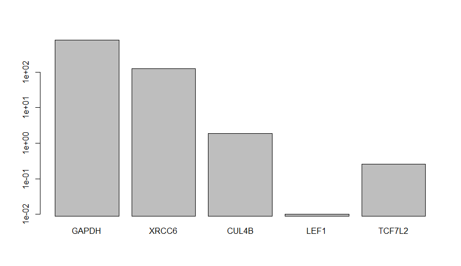
> barplot((results["RPKM",])+0.01,log="y")
> write.csv(results, "rpkm.csv")

The RPKM values were increased of 0.01 to allow bar-plotting in the log scale on the y-axis. As expected, GAPDH is the most expressed gene within the group of gene of interest. Even if the RPKM-based method of relative gene expression quantification is not extremely accurate, it can provide a decent idea of whether two transcript are expressed at a comparable level or not.

Code available at: https://github.com/dami82/bioinfo/blob/master/RPKM.tool.R